Where are Bobcats Happy?
Developing a new habitat suitability index for bobcats in Vermont
Although bobcats have a wide distribution of habitat across North America, the North American population has declined in recent decades due to increased agriculture and human development. While bobcat populations have remained fairly stable in Vermont, updating the map of bobcat habitat in Vermont will help conservation efforts with these famously secretive cats.
This study seeks to develop a habitat suitability index (HSI) for bobcat habitat in Vermont. A habitat suitability index is concept used in environmental science to model where various species could live based on different factors that shape habitat, such a where available food can be found, or preferred types of forest. By comparing a HSI with data of known bobcat sightings, the model can be tested and then hopefully applied for future habitat management.

Methodology
What criteria explain bobcat habitat?
The most recent Vermont Bobcat Study said that the top habitats for bobcats are forest, scrub/shrub, wetlands, and stream buffers, while they do not like agriculture, developed areas, and avoid roads (2017). The study also said that bobcats cannot hunt prey when snow is deeper than 8 inches. Attempts to model bobcat winter habitat in New Hampshire used the criteria of snow (max and average depth), elevation, land cover, aspect, slope, terrain ruggedness, distance to forest edge, distance to streams, distance to roads, road density, and traffic density (Reed, 2013). Boyle and Fendley focused on bobcat habitat in the southeast United States, with the primary variable being food (prey) availability (1987). Lastly, Preuss and Gehring constructed a habitat model based upon extensive field studies in northern Michigan; areas with high bobcat populations had higher percent forest, wetland, and stream cover, while bobcats avoided areas with high urban, open water, field, and transportation land cover types (2007). The criteria presented in these articles and the availability of relevant data were used to determine which criteria were incorporated in this study's model.
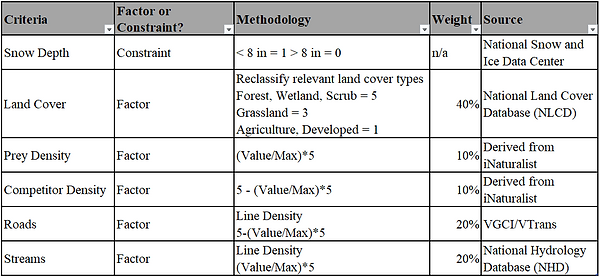
For this study, a mix of constraints and factors were used. Factors were ranked on or adjusted to a scale of 1 to 5, with 5 representing desirable habitats. The factors were combined in a weighted sum using raster calculator, which was then combined with the constraint to produce a habitat suitability index raster. The weighted sums were determined loosely based on the results of the coefficients generated by Reed’s model, with land cover type being more important than streams and roads, followed by the prey and competitor distribution (2013). The criteria used in this habitat suitability index are as follows:

,
Once the HSI raster was developed, it was compared with observed bobcat sightings in the area using regression in order to test the accuracy of the model. Bobcat sighting points, derived from iNaturalist, a citizen science website, were interpolated using a kriging algorithm to reduce the bias towards clusters of points. The bobcat sighting and HSI rasters were then resampled into a 500 x 500 m fishnet using zonal statistics in order to snap the rasters to a standard grid with a more appropriate grain size. The fishnet rasters were converted to polygons with integer values, and the bobcat polygons were joined to the suitability polygons using spatial join, with a median field mapping rule used to summarize the bobcat sightings. This layer combines all of the bobcat sighting and suitability data in one layer, which allows the regression tools in ArcGIS to be run.
Regression Results


GWR Results
Bandwidth = 6178.743329
ResidualSquares = 177.526749
Sigma = 0.516801
AICc = 1161.41599
R2 = 0.494644
R2Adjusted = 0.438145
Moran's I (OSL)
Moran's Index = 0.51560
z-score = 40.371140
p-value = 0.000000
Moran's I (GWR)
Moran's Index = 0.201873
z-score = 16.016529
p-value = 0.000000
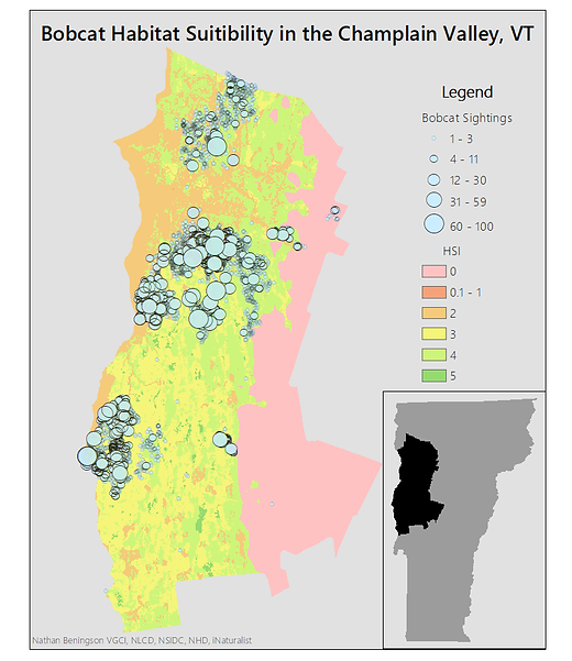
An ordinary least squares (OLS) regression was run, with suitability as the independent variable and bobcat sightings as the dependent variable. The results had a very high P-value and R-squared of almost 0, indicating that suitability does not have any significant relationship with bobcat sightings. A Moran’s I test was run on the residuals of the OLS to check for possible spatial autocorrelation. The Moran’s index of 0.51, z-score of 40, and P-value of 0 indicate that the data are significantly spatially clustered, and that a geographic weighted regression (GWR) is a more appropriate method. The GWR returned a R-squared value of 0.49, meaning that the HSI can explain 49% of the variation in bobcat sightings, a fairly strong value for this context. It is worth noting that there is a fairly high residual squares value of 178, indicating that the model does not fit the data that well, and a second Moran’s I test indicated that the GWR residuals are still spatially clustered, although not as much as the OLS residuals. The distribution of the GWR coefficients also appears to somewhat support the HSI, as the highest positive GWR coefficients overlap with with areas on the extremes of the HSI scale. Although the HSI model does not predict bobcat sightings with a high degree of accuracy, it appears to roughly indicate where bobcats may or may not live.
GWR Coefficients vs. HSI


Limitations
-
Some of the classifications, specifically land cover, were subjectively ranked on the 5-point scale and can only reflect the relative, not absolute, suitability of different criteria. The weights also suffer from a similar fault; although the relative weights were based on scientific research, the specific percentages were derived from the author’s intuition using round numbers. In general, it is difficult to reduce complex environmental processes into a 1 to 5 scale.
-
The interpolation of the bobcat point data into a raster surface resulting in some surprising results, likely due to a few points with very high number of sightings having an outsized impact on the interpolation. Although kriging seeks to reduce the influence of some of the clusters of points, the points seemed to cluster into three main groups, where a more even spread of bobcat sightings across the fairly similar landscapes of the Champlain Valley would be expected.
-
The bobcat sighting data originates from iNaturalist, a citizen science website, and data is likely biased towards more populated areas with more active respondents. The predator and competitor rasters were also derived using similar methods, and are therefore susceptible to similar biases in sampling and interpolation. The sighting may not actually reflect where the bobcats live.
-
When the HSI and bobcat sighting data were converted to polygons, they were first converted to integers in order to operate ArcGIS’s raster to polygon tool. This reduced the variation in the data, as both rasters were previously float data as a result of taking the average during the zonal statistics resampling into the fishnet.
-
The criteria may not be accurate predictors of bobcat habitat. Although these criteria were selected with respect to the location in western Vermont, certain criteria seemed to have more influence than first thought, such as riparian corridors. Bobcats were also observed in areas with snow that is theoretically too deep for them to hunt, meaning snow depth could have been treated as a factor instead of a constraint. Further regression analysis could better indicate to what extent different factors should be considered.
Management Implications
The management recommendations from the Vermont Fish and Wildlife Department are to maintain large buffers along rivers and streams for travel corridors, maintain undeveloped, connected blocks of habitat composed of desirable land cover, and to minimize fragmentation from roads (2017). Much of habitat conservation and management currently focuses on habitat connectivity (Crooks and Sanjayan, 2006), and incorporating bobcat habitat connectivity fits into greater habitat connectivity goals across the state for animals from black bear to spotted salamander. Riparian buffers also provide many other conservation benefits in addition to bobcat habitat. Road fragmentation also fits into the habitat connectivity discourse, but is especially relevant for Chittenden County, Vermont’s fastest growing and most densely populated county. Although bobcat populations in Vermont are fairly stable, unfettered development threatens their future habitats.
Works Cited
Boyle, K. A. (1987). Habitat suitability index models :bobcat /. Washington, DC : Retrieved from http://hdl.handle.net/2027/umn.31951d002829423
Crooks, K. R., & Sanjayan, M. (2006). Connectivity Conservation. Cambridge University Press.
Reed, G. C. (2013). Bobcats in New Hampshire: understanding the relationships between habitat suitability, connectivity and abundance in a changing landscape. MS Thesis, University of New Hampshire, Durham. Retrieved from http://mlitvaitis.unh.edu/Research/BobcatWeb/ProgressReports/Reed_Thesis.pdf
Roberts, S. B., Jordan, J. D., Bettinger, P., & Warren, R. J. (2010). Using Bobcat Habitat Suitability to Prioritize Habitat Preservation on a Suburbanizing Barrier Island. The Journal of Wildlife Management, 74(3), 386–394.
VT Fish and Wildlife. (2017). Bobcat Study in Vermont. Retrieved from http://www.vtfishandwildlife.com/